데분방01) Basics and R environment
Basics and R environment


📜 제목으로 보기✏마지막 댓글로
- 강의주소:https://lms.knou.ac.kr/dks/user/home/initUSTHomeIndex_GRSC.do?stLeftMenuId=0
- 선배블로그: https://insb.tistory.com/9?category=967351
- 작년 김성수 교수 강의로 진행
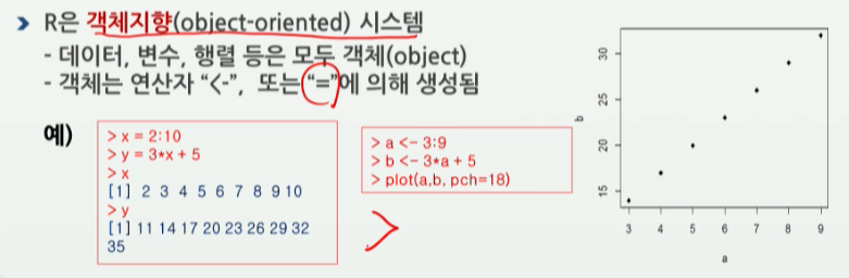
x = 2:10
x
y <- 3*x + 5
y
a <- 3:9
b <- 3*a + 5
plot(a, b)

plot(a, b, pch=18)


-
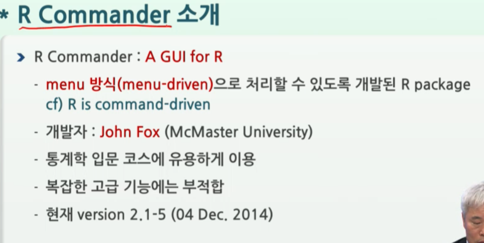
1980년대
S언어 탄생 by AT&T Bell Lab(c언어 개발한 연구소)에서 통계언어 S를 구현함- 1998 ACM S/W 상을 John Chambers가 탐 "Forever altered how people analyze, visualize and manipulate data
- 사람들이 어떻게 데이터 분석, 시각화, 다루는지를 영원히 바꾼 언어다
- 1998 ACM S/W 상을 John Chambers가 탐 "Forever altered how people analyze, visualize and manipulate data
-
오클란드 대학의 Ross and Robert 교수 2명이 S 축소버전인
R & R을 만듦 -
1995년 Martin Maechler(마틴 매흘러)가 R&R(이하카, 젠틀만)을 설득하여, linux처럼 오픈소스(GPL)로 쓰게 한 것인
R source code발표 -
1997년 8월
R core team결성. 2000년 02월 29일R version 1.0.0발표-
- 12월 R version 3.2.3
-
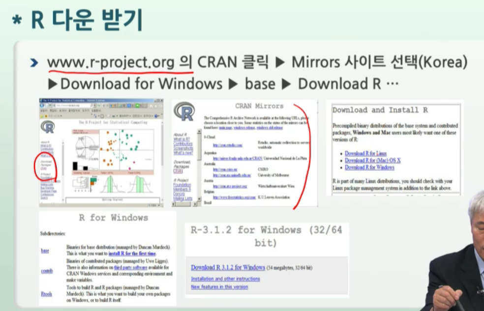
- base버전으로 다운 받기
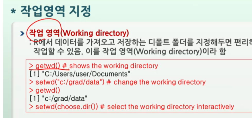
getwd()
setwd(".")
setwd( choose.dir() )
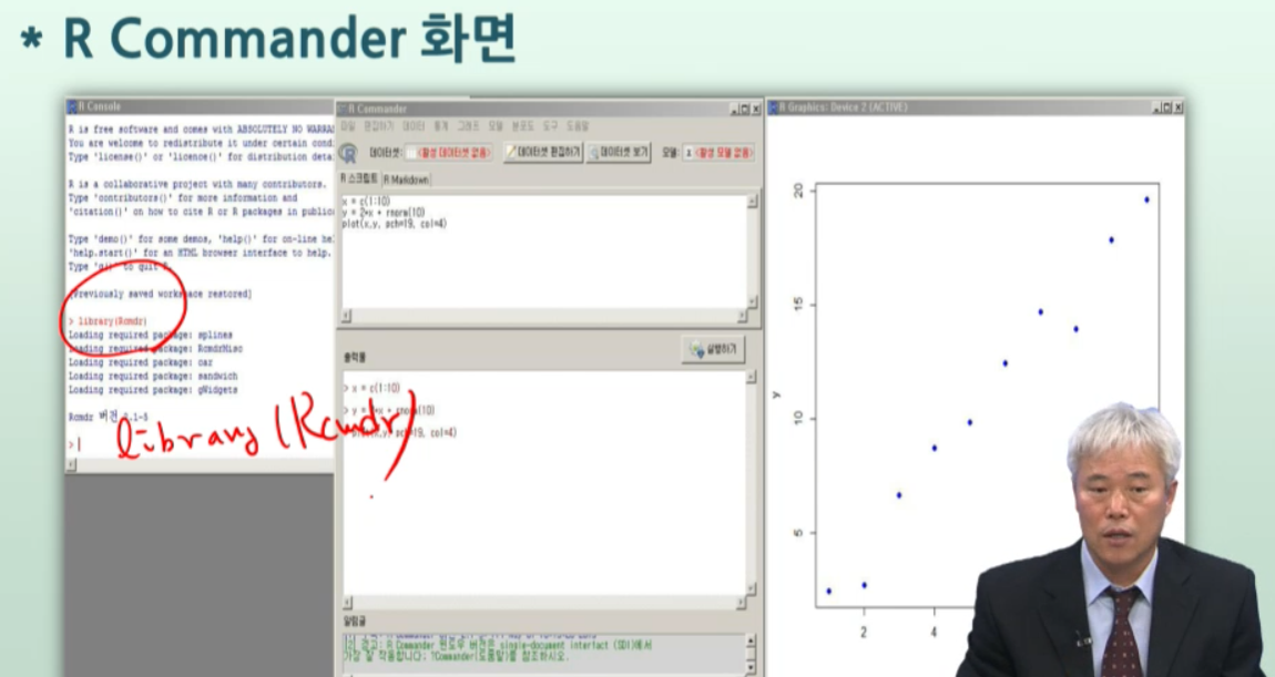
install.packages("ISwR")
library(ISwR)
plot( rnorm(1000), pch = 19)

weight <- c(60, 72, 57, 90, 95, 72)
height <- c(1.75, 1.80, 1.65, 1.90, 1.74, 1.91)
bmi <- weight/height^2
bmi
# 벡터c의 갯수 -> length( )
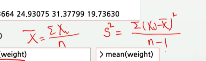
xbar <- sum(weight) / length(weight)
xbar
mean(weight)
sqrt(sum((weight-xbar)^2) / (length(weight) - 1))
sd(weight)
bmi
t.test(bmi, mu=22.5) # H0: mu=22.5 / H1: mu!=22.5

# t값 , 자유도, p값
# color="대or소문자" 대신 col=2번호를 줘도 된다. like pch=숫자
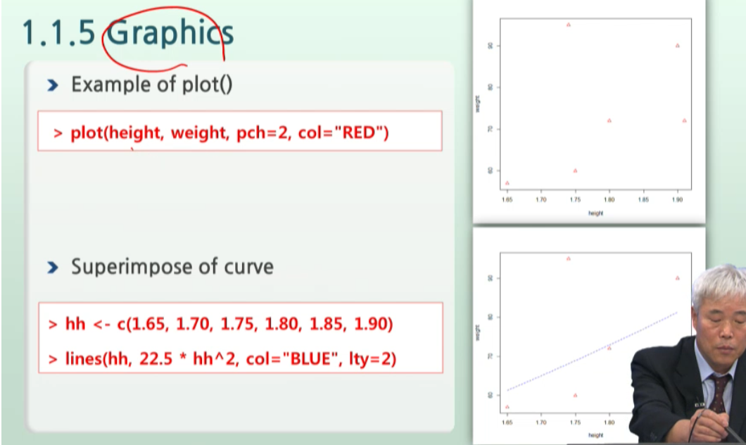
plot(height, weight, pch=2, col="RED")

# c벡터객체 1개 만들고
hh <- c(1.65, 1.70, 1.75, 1.80, 1.85, 1.90)
# lines로 선 그리기
lines(hh, 22.5*hh^2, col="BLUE", lty=2) # lty = line type -> 2번은 점점점 타입
plot(height, weight, pch=2, col="RED")

hh <- c(1.65, 1.70, 1.75, 1.80, 1.85, 1.90)
lines(hh, 22.5*hh^2, col="BLUE", lty=2)

# - 작따->큰따로 변환되서 표기된다.
# - 여기선 큰따-> 작따로 표기되네..like python
c("Huey", "Dewey", "Louie")
c('Huey', 'Dewey', 'Louie')
c(T, T, F, T)
bmi
# 벡터 + 조건식 -> 마스크가 된다.
bmi > 25
cat( c("Huey", "Dewey", "Louie") )
cat( c("Huey", "Dewey", "Louie", "\n") )
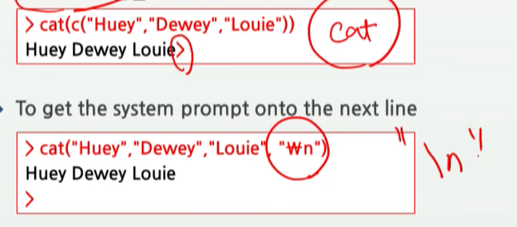
cat("What is \"R\"?\n")
예제 참고자료 사이트
- 예제 파일을 들고 있는 블로그: https://booolean.tistory.com/913?category=807312
wd <- read.table("./data//01/wd.txt", sep = "\t", header=T) # "./따옴표경로" , sep="구분자" , header=T (첫줄이 타이틀)
wd
nwd = wd

nwd
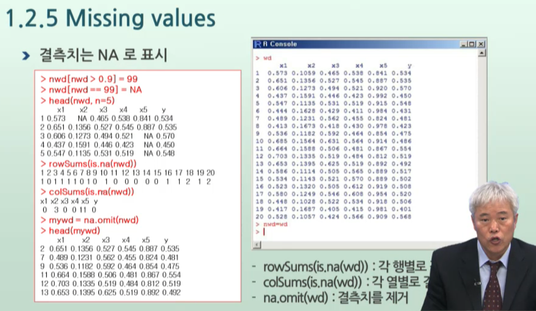
nwd[ nwd > 0.9 ] = 99
head(nwd)
nwd[nwd == 99] = NA

head(nwd)
# is.na()는 데이터객체 전체에 대한 boolean mask(logical character)를 만든다. -> 행렬mask -> 행 or 열별로 접근해줘야한다.
is.na(nwd)
rowSums( is.na(nwd) )
colSums( is.na(nwd) )
# -> 행별로 제거하는 듯 싶다.
# -> na.omit()의 결과 <기존 행번호>가 같이 찍히니 확인하면 된다.
na.omit(nwd)
nwd
x <- c(1,2,3)
y <- c(10, 20)

c(x, y, 5) # 벡터객체와 값이 동등하게 1차원으로 연결된다.
# boolean + 숫자 -> 숫자로 type 0/1로 바뀌어서 type통일
c(FALSE, 3)
c(FALSE, "abc")
c(pi, "abc")
seq(4, 9)
oops <- c(7, 9, 13)
rep(oops, 3)
# - index순서대로 1번, 2번, 3번 반복복사
# - index별 반복회수도 벡터로 제공하면 된다.
rep(oops, c(1,2,3))
rep(oops, 1:3)
rep(1:2, c(10, 15))
x <- 1:12
x
# 행렬이 된다.
dim(x) = c(3, 4)

x # 보이진 않지만, 1, 2, 3, 행    ,1 ,2 ,3 ,4 렬이 된다.
# - 특히 byrow=를 T루로 주면, ncol없이 알아서 된다.
matrix(1:12, nrow=3, byrow=T)
LETTERS[1:3]
rownames(x) <- LETTERS[1:3]
x
t(x)
# 1차원들을 -> 눕혀서 행으로 더하는 rbind

cbind(A = 1:4)
cbind(A = 1:4, B = 5:6, C = 9:12)
rbind(A=1:4,B=5:8,C=9:12)
aa <- cbind(A=1:4,B=5:8,C=9:12)
aa
# - 좌or우 똑같은 크기의 상수를 붙이려면 상수로 bind하면 된다.

cbind(1, aa)
pain <- c(0, 3, 2, 2, 1)
# -> levels=에는 [요인들과 동일한 값]으로 레벨을 정해서 매칭해놓는다.
# -> 연속적인 숫자벡터를 줬어도 '0'~'3'의 문자열로 정해진다.
# -> 매칭된 요인-레벨에 대해서, 레벨이름levels을 바꿔주면 요인들도 따라 바뀐다.

fpain <- factor(pain, levels = 0:3)

fpain
# -> 원본 값들이 레벨에 따른 해당 [라벨]로 바껴버린다.
levels(fpain) <- c("none", "mild", "medium", "severe")

fpain

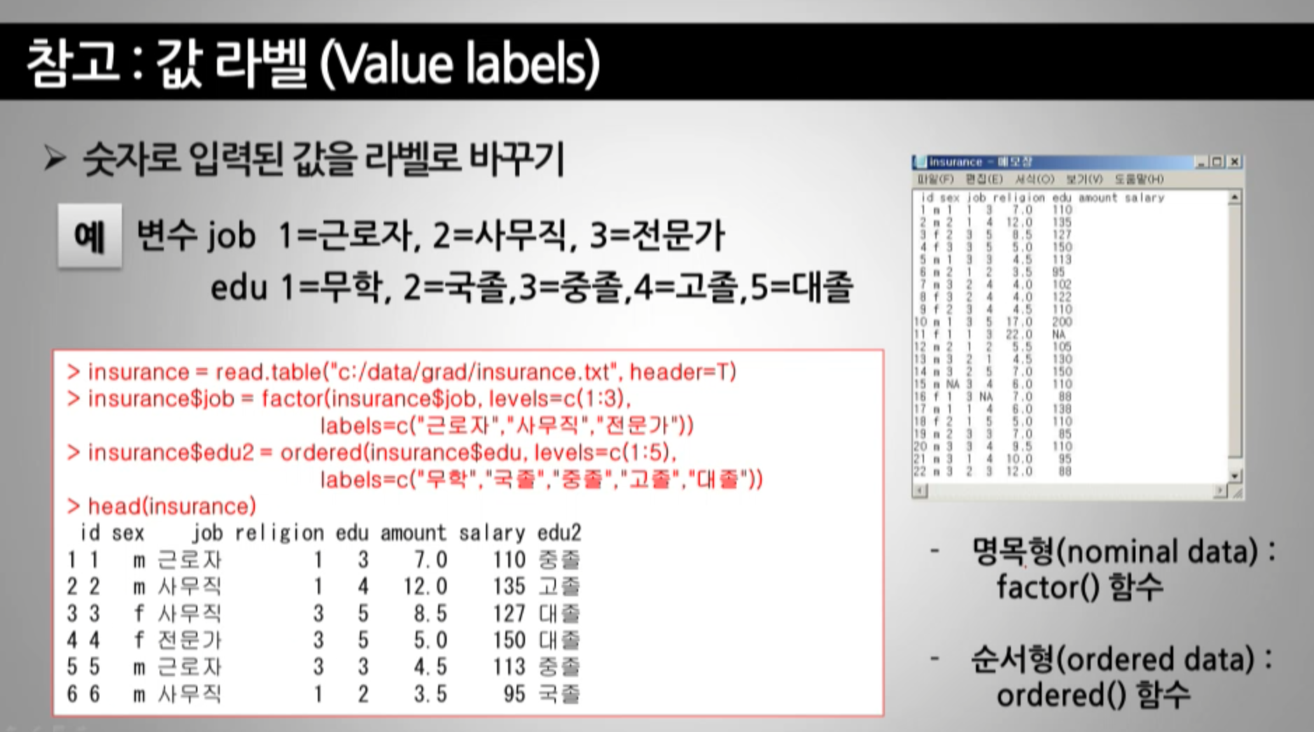
변수 job, edu를 숫자 -> 라벨(요인)으로 바꿔보자.
insurance = read.table("./data/01//insurance.txt", sep = "\t", header=T)
head(insurance)
insurance$job
insurance = read.table("./data/01//insurance.txt", sep = "\t", header=T,
                       na.strings = "-9")
insurance$job
# (3) 덮어쓸 labels도 순서대로 동시에 준다.
insurance$job <- factor(insurance$job,
       levels = 1:3,
       labels = c("근로자", "사무직", "전문가")
      )
insurance$job
head(insurance)
insurance$edu2 <-
factor(insurance$edu,
       levels = 1:5,
       labels = c("무학", "국졸", "중졸", "고졸", "대졸")
      )
insurance
intake.pre <- c(5260, 5470, 5640, 6180, 6390)
intake.post <- c(3910, 4220, 3885, 5160, 5645)
mylist <- list(before=intake.pre, after=intake.post)


mylist # df의 칼럼처럼 뽑아쓸 수 있게 모아준다.
mylist$before
d <- data.frame(intake.pre, intake.post)
d
d$intake.pre
intake.pre[c(1,5)]
intake.pre[- c(1,5)]
intake.post
intake.pre
# 1) [pre가 6000보다 컸]던 id의 환자들에 대해
# 2) post 수치는?
intake.post[ intake.pre > 6000 ]
intake.post[ intake.pre > 5500 & intake.pre <= 6200 ]
# - 비운 행or렬 = 전체
d [ d$intake.pre > 6000, ]
library("ISwR")
data(thuesen)
head(thuesen, 3) # 2개의 변수가 있는 데이터 투센
# - l을 붙이면, 각 변수들이 변수명을 가진 list()로 합쳐진다. like before=,after=
lapply( thuesen, mean)
# - na.rm = T : 미싱밸류를.제거한
lapply( thuesen, mean, na.rm = T)
# - 그냥 벡터형식으로 풀어진다.
sapply(thuesen, mean, na.rm = T)
# - 데이터를 바로 넣으면 안해준다.
# - (데이터변수 , 그룹변수, 집계)순으로 지정해줘야한다.
tapply(thuesen, mean, na.rm = T)
tapply(thuesen$blood.glucose, thuesen$short.velocity, mean, na.rm = T)
data(energy)
energy
tapply(energy$expend, energy$stature, mean, na.rm = T)
# - 1=row별 가로집계 / 2=col별 세로집계
m = matrix(rnorm(12), 4) # 2번째인자가 row수만 지정해주는 듯
m
# - 칼럼별 최소값
apply(m, 2, min)
intake
typeof(intake$post)
o1 <- order(intake$post)
o1
typeof(o1)
intake$post
# -> 해당칼럼에 대한 오름차순 order객체로 정렬
intake$post[o1]
intake$pre
intake$pre[o1]
ls()
rm(aa, b) # rm으로 데이터객체 삭제 -> 콤마로 한번에 여러개 가능
ls()
# df객체 속 변수를 바로 쓰는 방법은?
# -> session에 df자체를 attach해버리는 것 -> 가진 칼럼들이 다 변수로 붙어진다?
# --> 함수들의 인자로 넣기 쉽게 하기 위함인듯?
head(thuesen, 3)
attach(thuesen)
ls()
blood.glucose
# - 인덱싱과 마찬가진데, 함수를 쓴다.?!

thue2 <- subset(thuesen, blood.glucose < 7)
thue2
# - 로그값을 씌운 변수를 함수로 생성하여 반환
thue3 <- transform(thuesen, log.gluc = log(blood.glucose))
head(thue3, 4)
# -> 중괄호{}를 이용하여, 입력된 df내에서 변수생성/조작/중간변수 삭제가 가능하다.
thue4 <- within(thuesen, {
            log.gluc <- log(blood.glucose) # + log씌운 칼럼 생성
            m <- mean(log.gluc) # 평균값 계산(중간변수)
            centered.log.gluc <- log.gluc - m # 중간변수를 이용해 새로운 칼럼 추가 생성
            rm(m)
        })


head(thue4)
x <- runif(50,0,2)
y <- runif(50, 0,2)
plot( x, y,
     main="Main title",
     sub="subtitle",
     xlab="x-label",
     ylab="y-label",
    )

# -> x, y좌표에 텍스트를 넣어준다.
text(0.6, 0.6,
    "text at (0.6, 0.6)")
plot( x, y,
     main="Main title",
     sub="subtitle",
     xlab="x-label",
     ylab="y-label",
    )

text(0.6, 0.6,
    "text at (0.6, 0.6)")

abline(h=.6, v=.6, lty=2)
plot( x, y,
     main="Main title",
     sub="subtitle",
     xlab="x-label",
     ylab="y-label",
    )

text(0.6, 0.6,
    "text at (0.6, 0.6)")

abline(h=.6, v=.6, lty=2)

# ->  -1부터 4숫자를, 각 side에 , 0.7크기로, -1~4의 위치에 적기
for (side in 1:4)
    mtext(-1:4, side=side, at=.7, line=-1:4)
plot( x, y,
     main="Main title",
     sub="subtitle",
     xlab="x-label",
     ylab="y-label",
    )

text(0.6, 0.6,
    "text at (0.6, 0.6)")

abline(h=.6, v=.6, lty=2)

for (side in 1:4)
    # -1부터 4숫자를, 각 side에 , 0.7크기로, -1~4의 위치에 적기
    mtext(-1:4, side=side, at=.7, line=-1:4)

c(1:4)
1:4
mtext(paste("side", 1:4), side=c(1:4), line=-1, font=2)
plot( x, y,
     main="Main title",
     sub="subtitle",
     xlab="x-label",
     ylab="y-label",
    )

text(0.6, 0.6,
    "text at (0.6, 0.6)")

abline(h=.6, v=.6, lty=2)

for (side in 1:4)
    mtext(-1:4, side=side, at=.7, line=-1:4)

mtext(paste("side", 1:4), side=c(1:4), line=-1, font=2)

plot(x, y)

# -> 흰색으로 표시만 지우고 도화지만 그려놓는다는 의미

# 라벨도 ""로 다 지우고

# axes= F -> 축도 그리지 말고 있어라.

plot(x, y,
     type="n",
     xlab="", ylab="",
     axes=F
     )

plot(x, y,
     type="n", xlab="", ylab="", axes=F)

points(x, y)

# 2) axis(1) -> 1번 축(x축)만 그려라
plot(x, y,
     type="n", xlab="", ylab="", axes=F)

points(x, y)
axis(1)

# 2) axis(1) -> 1번 축(x축)만 그려라
# 3) axis(2, at= ) -> 2번 축(좌 y축)에는 점을 직접 찍어준다.


plot(x, y,
     type="n", xlab="", ylab="", axes=F)

points(x, y)
axis(1)
axis(2, at=seq(0.2, 1.8, 0.2))

# 2) axis(1) -> 1번 축(x축)만 그려라
# 3) axis(2, at= ) -> 2번 축(좌 y축)에는 점을 직접 찍어준다.
# 4) box() -> 4방향 축이 사각형으로 모두 그려진다.

plot(x, y,
     type="n", xlab="", ylab="", axes=F)

points(x, y)
axis(1)
axis(2, at=seq(0.2, 1.8, 0.2))
box()

# 2) axis(1) -> 1번 축(x축)만 그려라
# 3) axis(2, at= ) -> 2번 축(좌 y축)에는 점을 직접 찍어준다.
# 4) box() -> 4방향 축이 사각형으로 모두 그려진다.
# 5) title() ->  main(위) sub(아래)  xlab, ylab -> 2개 축 라벨

plot(x, y,
     type="n", xlab="", ylab="", axes=F)

points(x, y)
axis(1)
axis(2, at=seq(0.2, 1.8, 0.2))
box()
title(main="Main title", sub = "subttitle",
      xlab="x-label", ylab="y-label")

?par
par(mfrow=c(2,2)) # 한 화면을 2x2 로 나눠서 그린다.
par(mfrow=c(1,1))
# - 안주면 각각의 그림이 2개로 나눠서 각각 그려진다.


x <- rnorm(100) # 정규분포(r norm)를 따르는 놈 100개

hist(x, freq=F) # 히스토그램: freq=F 를 주면 빈도대신 비율(밀도)가 y축을 차지한다.
curve(dnorm(x), add=T) # 정규분포 함수dnorm(x) 를 curve로 그리는데, 겹쳐서 그려라 add=T

# my) 정규분포 변수 -> rnorm(갯수)
# my) 정규분포 함수 -> dnorm(변수)

# 다시 그리고 -> add=T로 2번째 그림 그리고


h <- hist(x, plot=F)
h
h <- hist(x, plot=F)

# 기존 hist plot 객체에서 y축 정보만 가져와 -> 조작후 객체로 만든다.
ylim <- range(0, h$density, dnorm(0))

# 조작된 ylim으로 새로운 hist를 그린다.
hist(x, freq=F, ylim=ylim)

curve(dnorm(x), add=T)

# -> 이후 파일로 저장하기 위해 스트링으로 바꿈
func_string <- "hist.with.normal <- function(x)
{
    hist <- hist(x, plot=F)
    s <- sd(x)
    m <- mean(x)
    ylim <- range(0, h$dentisy, dnorm(0, sd=s))

    hist(x, freq=F, ylim=ylim)
    curve(dnorm(x, m, s), add=T)
}"
filename <- "./01_p44.r"

fileConn <- file(filename)

writeLines(func_string, fileConn)
close(fileConn)
source(filename)
ls()
x <- rnorm(100)

hist.with.normal(x)

y <- 12345

# 1. while (조건) 식 으로 구하는 root
x <- y/2
while (abs(x*x-y) > 1e-10 ) x <- (x + y/x)/2

x
x^2
# 1. while (조건) 식 으로 구하는 root
# 2. repeat { 식  if 탈출조건 break}

repeat{
    x <- (x + y/x)/2
    if (abs(x*x-y) < 1e-10) break
}

x
x <- seq(0, 1, 0.5)

plot(x, x, ylab="y", type="l")

for ( j in 2:8 ) lines(x, x^j)

2.4 Data entry
- 김성수 2015 강의교안 저장된페이지
-
01 2015자료 데이터시각화.pdf에 코드 검색됨
-
textfile: read.table, read.csv -
excelfile : read.xlsx( package: xlsx)
install.packages("xlsx“)
library(xlsx)
drug.data = read.xlsx("c:/Rfolder/data/drug.xlsx", 1) # 1은 default인데, sheet번호다.
edit(drug.data) # R전용 데이터에디터에 가져와서 조작하고 싶을 때
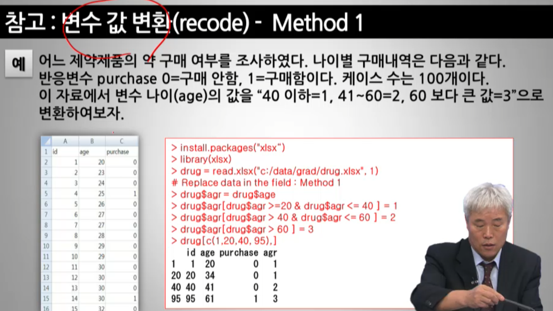
- (범위별 매핑 -> )
recode=변수 값 변환이라고 한다.
- 새 변수를 만들고 (할당으로 복사)
- 인덱싱을 이용해서 범위별로 값 변환
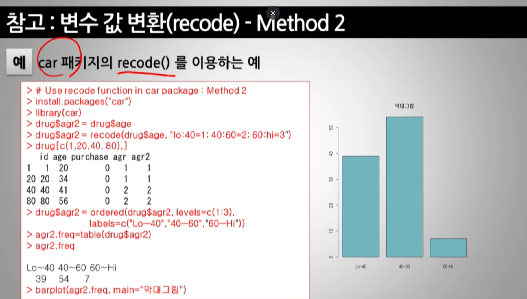
- 새 변수 만들어놓는 것은 똑같고
-
recode()함수를 이용하여범위를 간단하게 표현할 수 있다.- "
lo:40=1;40:60=2;60:hi=3"
- "
-
1,2,3 범주형 자료이면서 순서형 변수 순서를 ordered()를 이용해서 factor-라벨로 준다.
- 라벨을 주면 그래프에서도 나온다.