데분방03-1) One and Two sample Test
One and two-sample tests


📜 제목으로 보기✏마지막 댓글로
- 강의소개
- One- and two-sample tests
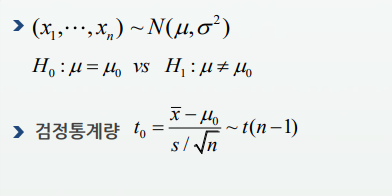
일표본 t 검정방법
독립표본 t 검정방법
대응표본 t 검정방법
Chapter 5. One- and two-sample tests
- 5.1 One-sample t test
- 5.2 Wilcoxon signed-rank test
- 5.3 Two-sample t test
- 5.4 Comparison of variances
- 5.5 Two-sample Wilcoxon test
- 5.6 The paired t test
- 5.7 The matched-pairs Wilcoxon test
# -> remcommend되는 량이 7725 kJ인데
# -> 11개 데이터는 평균이 == 뮤제로(7725kJ)인지 검증해보기

# H0: m == 7725
# H1: m != 7725  -> 자연스럽게 양측검증이된다.

# cf) H1: m < 7725 -> 단측검증
daily.intake <- c(5260,5470,5640,6180,6390,6515, 6805,7515,7515,8230,8770)
daily.intake
# -> 실제 평균 등의 숫자데이터의 mean() + sd() + 중앙값by quantile() + @ (boxplot, hist) 각각 구해보기
mean(daily.intake)

# -> 평균은 7725보단 작네
sd(daily.intake)

# -> 변동까지 고려할땐 sd구하기
quantile(daily.intake)

# -> 중앙값을 봤을 때도, 7725보다 작을 것을 예상
t.test(daily.intake, mu=7725)

# - t값, 자유도, p값=유의확률=0.01814 -> 유의수준a=0.05 기준    p값 < a보다 더 작아서
# --> 귀무가설 기각 reject H0

# true mean is not equal to 7725 : 양측검증을 기본으로 하는 일표본t검정

# 95% 신뢰구간 => 평균이 95% 확률로 여기있는 구간 ->   5986.348 < < 7520.925    7755보다 작은 곳에 95% 평균이 존재함
# --> 이 구간만 봐도, 귀무가설 기각되겠구나 알 수 있다.


# data deviate significantly(하게 벗어난다)from the hypothesis that the mean is 7725.
#  : mu (def=0), -> # mu=값을 안주면 0으로 검정하게 된다.


#  alternative = “grater”(“g”) or “less” (“l”) (def=two-sided),
# -> 단측검정으로서 <<h1기준>> mu보다 크다 검정 -> alternative ="g"옵션    vs  mu보다 작다 검정 alternative ="l"옵션
t.test(daily.intake, mu=7725, alternative = "l") # H1: m < 7725
# --> 단측검정의 p-value는 양측검증 p-value/2만 해주면 그 값이다

#  conf.level = 0.99 (def=0.95)
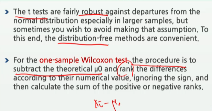
wilcox.test(daily.intake, mu = 7725)

# V값은 양수ranks들의 합이며, 통계량의 p-value는..
library("ISwR")

data(energy)
energy$stature # 범주칼럼 -> 범주의 종류 = 그룹의 갯수 -> 2종류 == 2그룹
# t.test(expend ~ stature)

# stature의 2그룹(2값)에 따라서 expend의 평균비교를 t.tset로 하시오
# -> y ~ x(그룹변수, 범주칼럼)
# H0: m1=m2, H1: m1 != m2

t.test(expend ~ stature, data=energy)

# 맨마지막에 각 그룹의 평균이 나옴

# 두 그릅의 평균을 뺀 뒤 표준화한 값이 t통계량 ->
# -> t0 = -3.85

# df= 15.919 -> 자유도 소수점이하로 나온다? -> 분산을 서로 다르다고 보고 작업하는 구나
# -> r에서 기본 제공하는 t-test인 Welch 독립표본 t-test는 2그룹간의 분산을 서로 다르다고 보고 있구나 생각

# p <0.05 : H0기각, H1채택 -> mean차이가 유의미하게 난다.
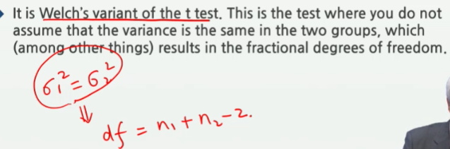
t.test(expend~stature, var.equal=T)
# df = n1 + n2 - 2

# p-value도 등분산성 가정안했을때보다 더 줄어든다.
# H0: 시그마1^2 = 시그마2^2

var.test(expend ~ stature, data=energy)

# 유의수준을 0.05가 아니라 0.1보다 작은지를 많이 쓴다.***

# 등분산성은 H0를 기각하지못해야 이득
# -> H0: 시그마1^2 = 시그마2^2  기각X -> 등분산성 증명된다.

# 등분산성을 만족시킨다면 -> t.test( , var.equal=T)로 평균이 같은지 검정한다.
wilcox.test(expend ~ stature, data=energy)

# p가 0.05보다 작으니 2그룹간에 차이가 있구나를 증명할 수 있다.

# W값은, 첫번째 그룹의 rank의 합이다.
intake # row개인별, 같은 표본으로서, 먹기 전/후 값
t.test(intake$pre, intake$post, paired = T)

# df = 10 -> 총 데이터 11개
# t-통계량 = 11 -> 엄청 크다 -> 차이가 확실히 있구나( t통계량은 평균을 빼서 표준화한 것?)
# e-07 -> 10^-7승
wilcox.test(pre, post, data=intake, paired=T)
wilcox.test(intake$pre, intake$post, paired=T)